Looking for the ultimate Google Sheets reference guide specifically designed for sales professionals? This Google Sheets cheat sheet covers all the essential formulas and features you need to manage prospects, track your pipeline, and analyze sales performance—all tailored to real-world sales scenarios.
For a complete reference of all Google Sheets functions, you can also check the official Google documentation.
AVERAGE, AVERAGEIF & AVERAGEIFS: Calculate key sales metrics and performance indicators
These functions help you understand typical values in your sales data, from deal sizes to conversion rates, and return the numerical average value rounded to the nearest integer when needed.
AVERAGE syntax
Start each formula with an equal sign (=), followed by the function name:
- =AVERAGE(range) – average of all values
- =AVERAGEIF(range, criteria, [average_range]) – average if one condition is met
- =AVERAGEIFS(average_range, criteria_range1, criteria1, …) – average with multiple conditions
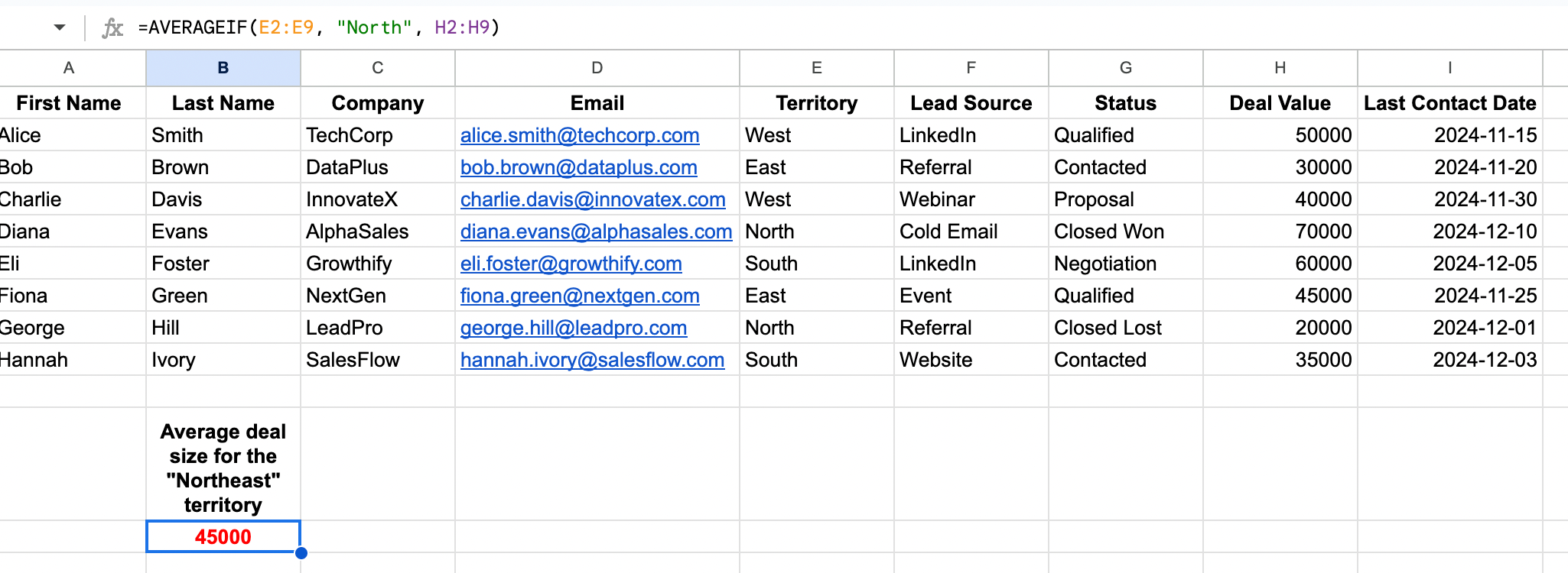
Sales example: Get the average deal size for the “North” territory:
=AVERAGEIF(E2:E9, "North", H2:H9)This returns the numerical average value in column H (deal amounts), but only for rows where column E (Territory) contains “North”.
Additional uses:
- Track average response time by lead source
- Measure average days to close by deal type
- Calculate average conversion rates by campaign
ARRAYFORMULA syntax
ARRAYFORMULA lets you perform calculations across entire ranges at once, eliminating the need to copy formulas down columns.
ARRAYFORMULA syntax:
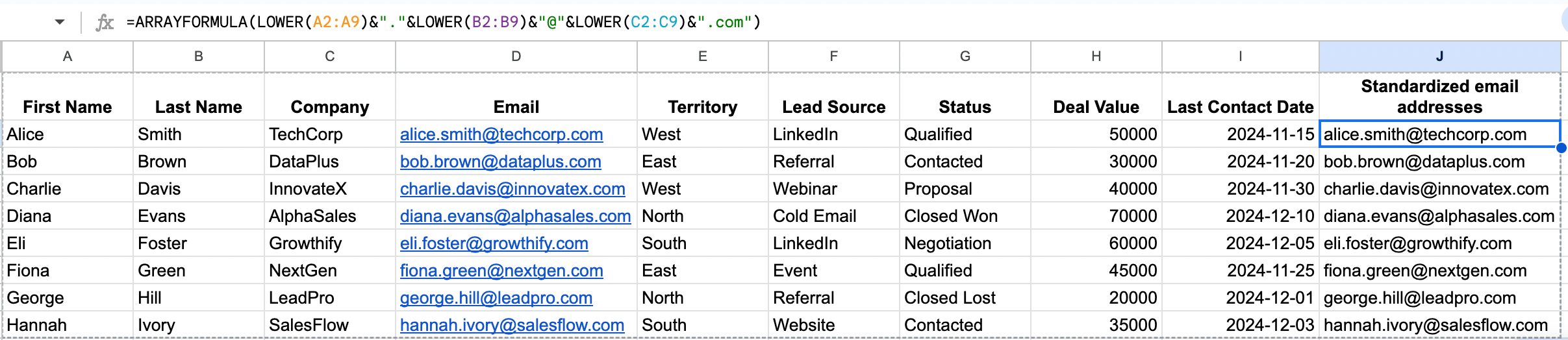
=ARRAYFORMULA(array_formula)Sales example: Create standardized email addresses for all prospects in one formula:
=ARRAYFORMULA(LOWER(A2:A100)&"."&LOWER(B2:B100)&"@"&LOWER(C2:C100)&".com")This takes first names (A2:A100), last names (B2:B100), and company names (C2:C100) to generate email addresses in format firstname.lastname@company.com
Additional uses:
- Calculate commission on every deal in your sales pipeline
- Create standardized tracking IDs for all prospects
- Apply lead scoring formulas to your entire database at once
CONCATENATE & CONCAT: Combine fields for cleaner prospect tracking
Whether you’re prepping a contact list or syncing to your CRM, these formulas help you combine data fields from multiple cells like names, company, or job title into one clean string.
CONCATENATE & CONCAT syntax:
- =CONCATENATE(text1, [text2], …) – Joins multiple text strings
- =CONCAT(text1, [text2], …) – Newer version with same functionality
- =text1&text2&text3 – Alternative using the ampersand operator
Tip: You can also use TEXTJOIN for more complex cases with delimiters.
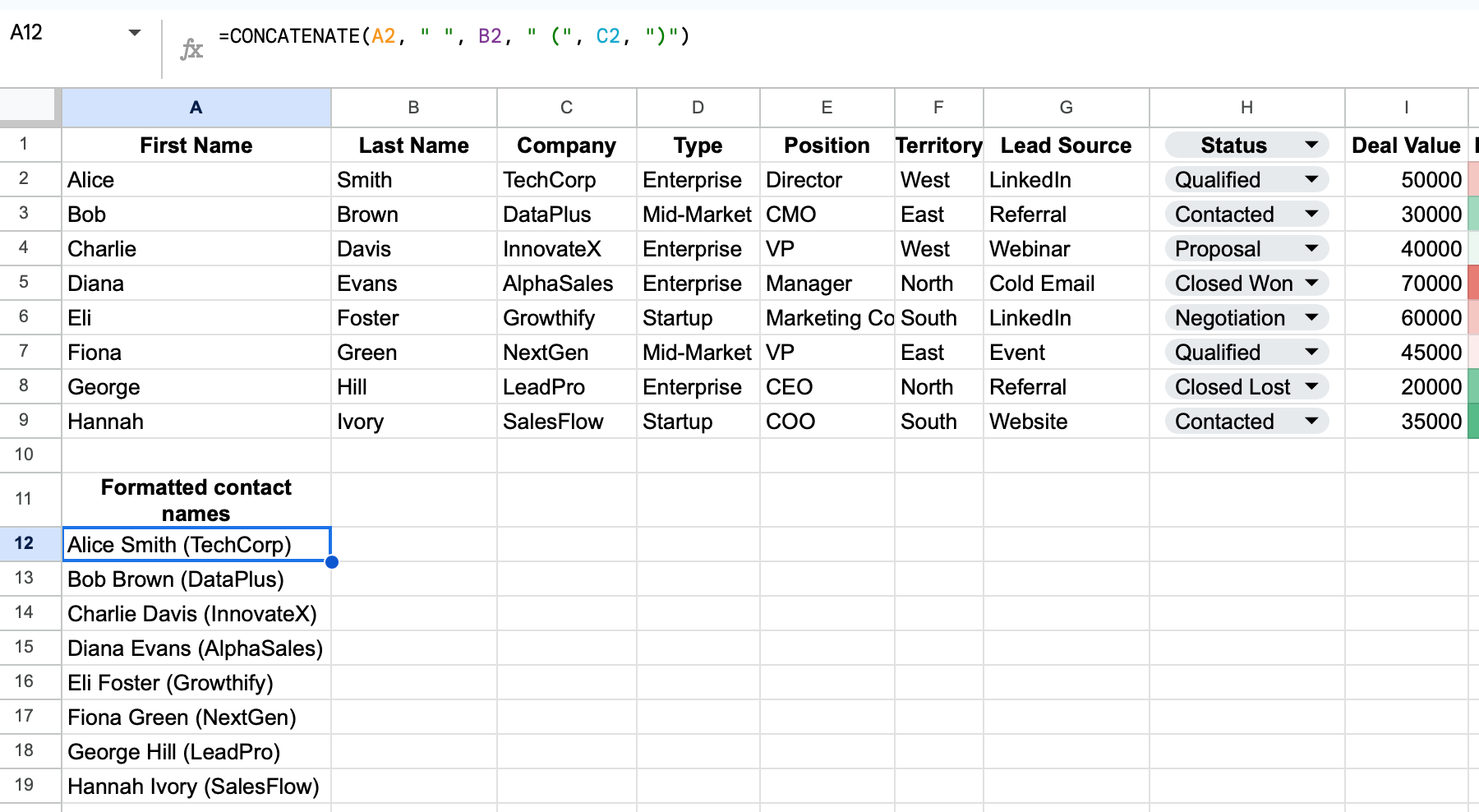
Sales example: Create a full name field for export
Let’s say your columns are:
- A = First name
- B = Last name
- C = Company
Option 1: Combine manually (one row at a time)
Use this if you’re working with a short list.
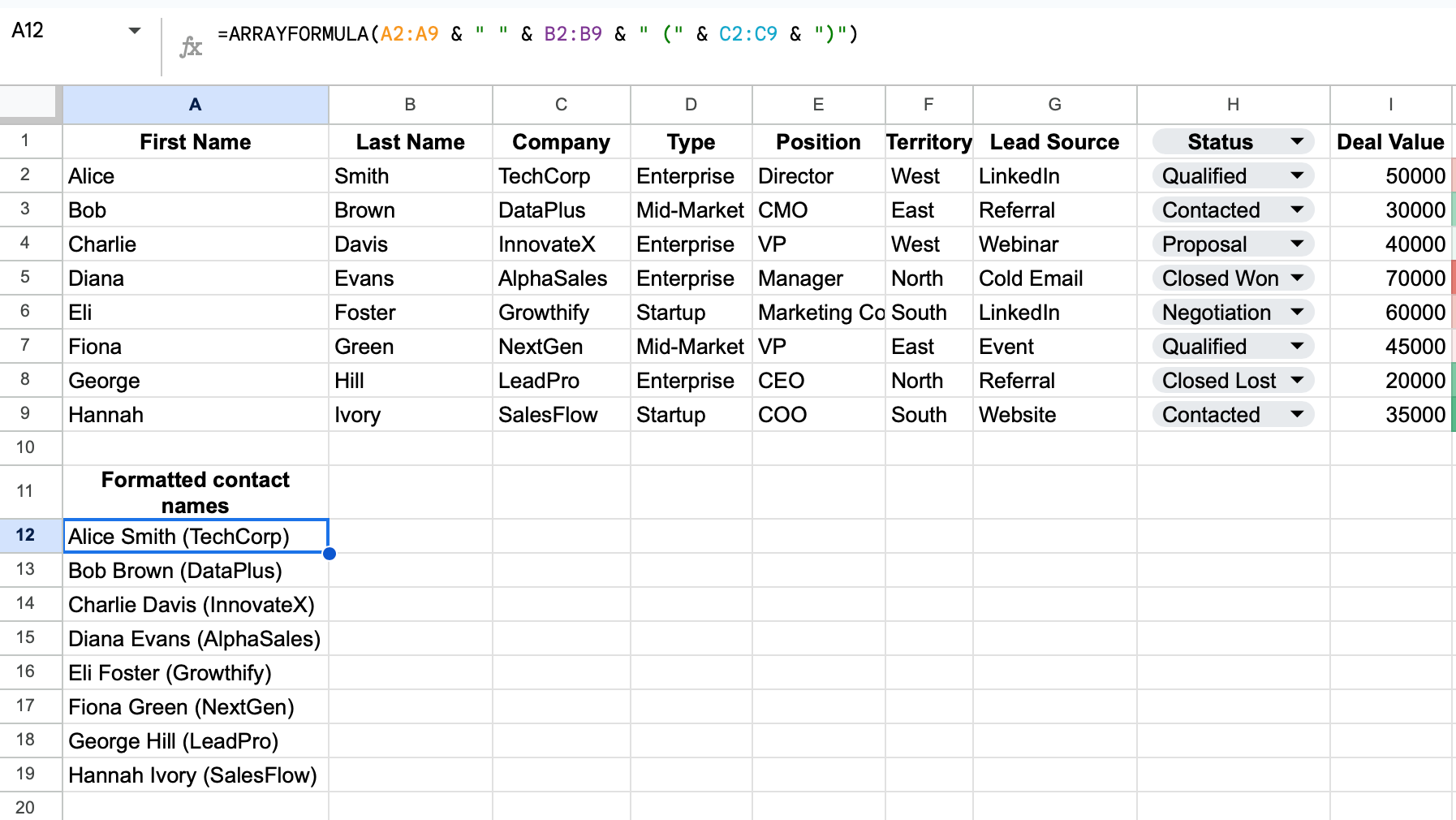
=CONCATENATE(A2, " ", B2, " (", C2, ")")This formula takes first name (A2), last name (B2), and company (C2) to generate something like: Alice Smith (TechCorp)
Option 2: Combine automatically with ARRAYFORMULA
Use this when working with longer lists or dynamic data.
=ARRAYFORMULA(A2:A & " " & B2:B & " (" & C2:C & ")")Same output, but for every row at once.
Additional uses:
- Standardize contact names before syncing with a CRM integration
- Create dynamic tags for segmentation in your prospect data management workflows
- Make your sales spreadsheet easier to scan, filter, or export
COUNT, COUNTA, COUNTIF & COUNTIFS: Track your leads and activities by category
These formulas help you count deals, contacts, or actions based on custom criteria, such as deal status, lead source, or a specified value. It’s perfect for understanding pipeline health, campaign results, or rep activity.
COUNT, COUNTA, COUNTIF & COUNTIFS syntax:
- =COUNT(range) — Counts numeric values in cells
- =COUNTA(range) — Counts non-empty cells
- =COUNTIF(range, criteria) — Counts cells in a specified range that match a given value
- =COUNTIFS(criteria_range1, criteria1, [criteria_range2, criteria2]…) — Counts based on multiple conditions
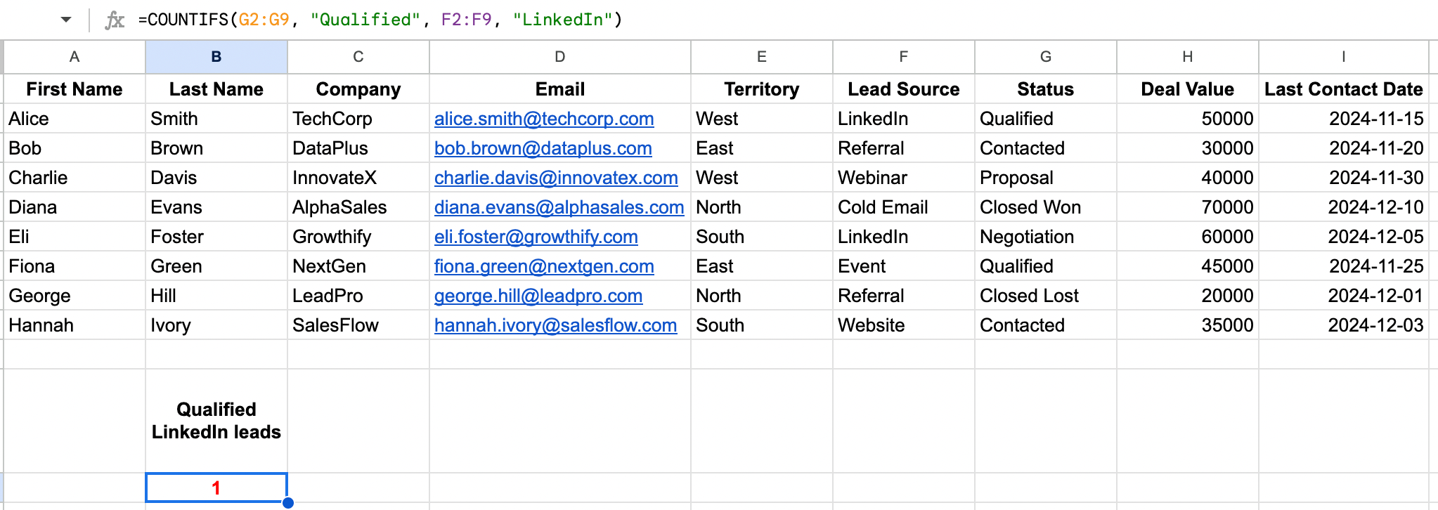
Sales example: Count qualified LinkedIn leads:
=COUNTIFS(G2:G9, "Qualified", F2:F9, "LinkedIn")This counts all rows where column G = “Qualified” and column F = “LinkedIn”, ideal for tracking lead source performance.
Additional uses:
- Track outreach attempts by sales rep
- Measure follow-up completion rates
- Count leads by source or industry
- Calculate conversion rate between pipeline stages
DATE, TODAY & NOW: Manage timelines and sales cycle duration
These functions help you calculate how long deals have been open based on the date value in each row.
DATE, TODAY & NOW syntax:
- =TODAY() – Returns the current date
- =NOW() – Returns the current date and time
- =DATE(year, month, day) – Creates a date from individual components
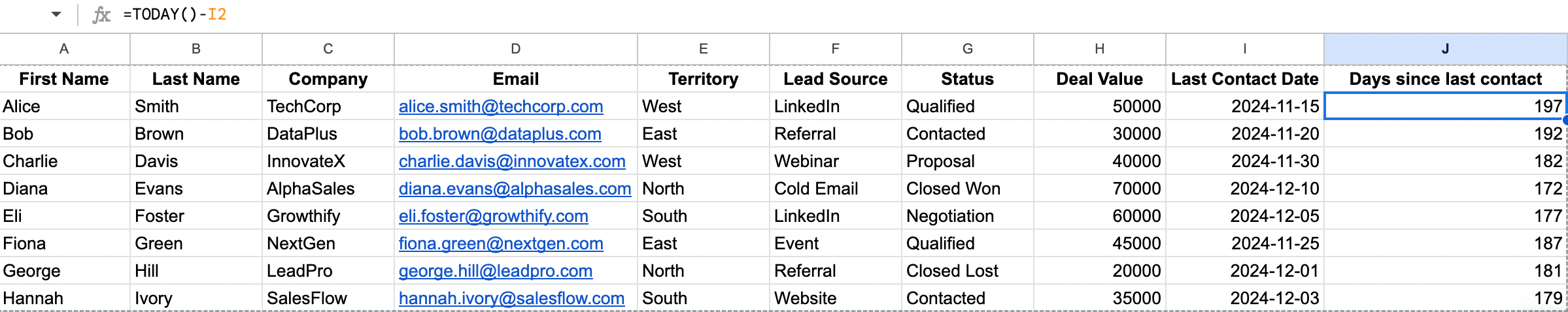
Sales example: Calculate days since last contact with prospects:
=TODAY()-F5Subtracts the date in cells from column F (last contact) from today’s date to get days elapsed
Additional uses:
- Prioritize outreach based on last touch or last meeting
- Combine with IF to tag leads as “cold” after X days
- Filter your sales pipeline by stage age or response delays
FILTER: Extract high-value prospects based on multiple criteria
FILTER helps you create dynamic lists of prospects that meet specific criteria, perfect for targeted outreach campaigns.
FILTER syntax:
=FILTER(range, condition1, [condition2, ...])Sales example: Extract high-value leads with recent engagement:
=FILTER(A2:I59, E2:E50 = "West", I2:I50 >= TODAY() - 30)
This returns all rows where Territory = “West” and Last Contact Date is within the past 30 days—ideal for follow-up campaigns.
Additional uses:
- Create call lists based on stage, value, or engagement
- Flag stalled deals that haven’t moved in weeks
- Filter your pipeline by industry, owner, or deal size
FIND & SEARCH: Locate key information in your prospect database
Need to build a targeted call list or flag promising leads for a campaign? FILTER helps you extract only the rows that match specific conditions, perfect for real-time segmentation.
FIND & SEARCH syntax:
- =FIND(find_text, within_text, [start_at]) — Case-sensitive
- =SEARCH(find_text, within_text, [start_at]) — Case-insensitive
For multiple keywords, use REGEXMATCH instead (see below). When working with text, wrap string conditions (e.g. “Qualified”) in quotation marks.
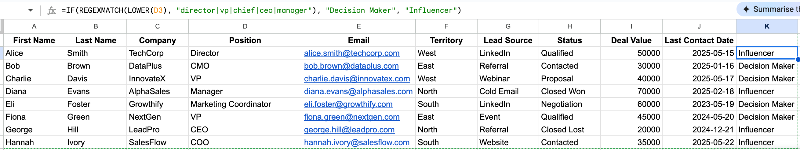
Sales example: Check if prospect titles indicate decision-making authority:
=IF(REGEXMATCH(LOWER(D3), "director|vp|chief|ceo|manager"), "Decision Maker", "Influencer")This checks if column D (e.g. job title) contains keywords that typically indicate decision authority. LOWER() ensures the match works regardless of case
Additional uses:
- Identify prospects mentioning specific pain points in notes
- Extract domain names from email addresses
- Check if company descriptions include target keywords
- Flag records containing specific information
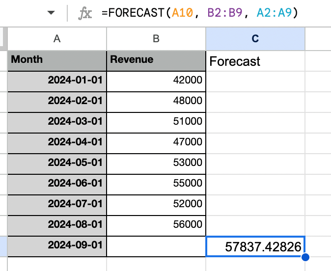
FORECAST: Predict sales outcomes and closing probabilities
FORECAST helps you project future results based on existing data, perfect for sales predictions and pipeline analysis. Calculate future value of projected deals
FORECAST syntax:
=FORECAST(x, known_y's, known_x's)Sales example: Project monthly closing values based on historical performance:
=FORECAST(A10, B2:B9, A2:A9)Calculate the future value of projected deals for the date in A10 based on historical values (B2:B9) from previous dates (A2:A9).
Additional uses:
- Predict resource needs for upcoming quarters
- Forecast lead volume based on marketing activities
- Calculate net present value of large deals
- Estimate close dates for complex sales cycles
- Project territory performance against targets
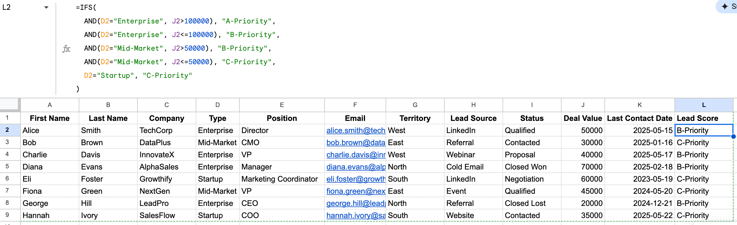
IF, IFS & IFERROR: Build lead scoring and qualification systems
These conditional functions let you return one value if true, another if false, to automate decisions in your sales process.
IF, IFS & IFERROR syntax:
- =IF(logical_test, value_if_true, value_if_false) – Basic conditional
- =IFS(condition1, value1, condition2, value2, …) – Multiple conditions
- =IFERROR(value, value_if_error) – Handle errors gracefully
Sales example: Create a lead scoring system:
=IFS(
    AND(D2="Enterprise", J2>100000), "A-Priority",
    AND(D2="Enterprise", J2<=100000), "B-Priority",
    AND(D2="Mid-Market", J2>50000), "B-Priority",
    AND(D2="Mid-Market", J2<=50000), "C-Priority",
    D2="SMB", "C-Priority"
)
Assigns priority ratings based on company type (D) and potential value (J)
Additional uses:
- Build logic for territory assignment
- Create deal stage advancement criteria
- Design automated qualification workflows
- Build custom status indicators for pipeline visualization
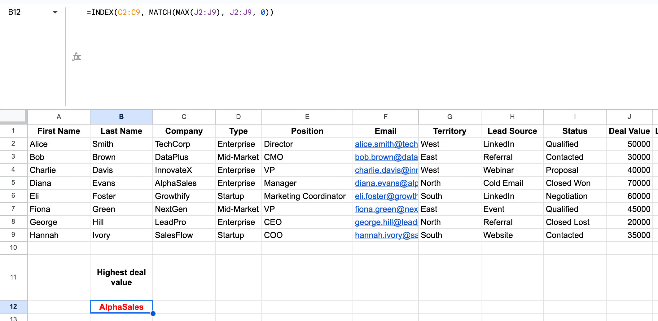
INDEX & MATCH: Create flexible lookups across multiple data points
This powerful combination provides more flexible lookups than VLOOKUP, using both row and column cell references
INDEX & MATCH syntax:
=INDEX(range, MATCH(lookup_value, lookup_range, 0))Sales example: Find the highest-performing sales rep for a specific industry:
=INDEX(C2:C100, MATCH(MAX(J2:J100), J2:J100, 0))This formula looks at the Deal Value column (J), finds the max value, and returns the corresponding value from column C.
Additional uses:
- Create two-way verification systems for data accuracy
- Build complex dashboards with dynamic reference points
- Perform lookups based on multiple criteria
- Create custom territory assignment systems
IMPORTRANGE: Connect team data without disrupting individual Workflows
IMPORTRANGE lets you pull data from other spreadsheets, perfect for creating centralized dashboards while team members maintain their own sheets.
IMPORTRANGE syntax:
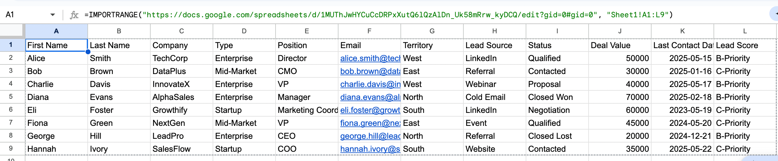
=IMPORTRANGE("spreadsheet_url", "range_string")⚠️ The first time you use IMPORTRANGE, Google Sheets will ask you to “Allow access” to connect the two files.
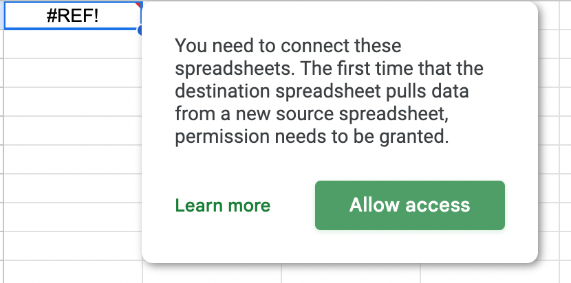
Sales example: Create a team dashboard pulling from individual rep spreadsheets:
=IMPORTRANGE("spreadsheet_url", "Sheet1!A1:L9")Imports data from the “Sheet1” tab, range A1:L9, from another spreadsheet using IMPORTRANGE().
Additional uses:
- Pull data from marketing campaigns into sales sheets
- Create management views without disrupting individual workflows
- Maintain separate territory sheets that feed into a master dashboard
- Connect lead generation data with sales activity tracking
LEFT, RIGHT & MID: Extract and parse contact information efficiently
These text functions extract portions of text strings, perfect for standardizing and parsing inconsistent data.
LEFT, RIGHT & MID syntax:
- =LEFT(text, num_chars) – Extracts characters from the start
- =RIGHT(text, num_chars) – Extracts characters from the end
- =MID(text, start_position, num_chars) – Extracts characters from the middle
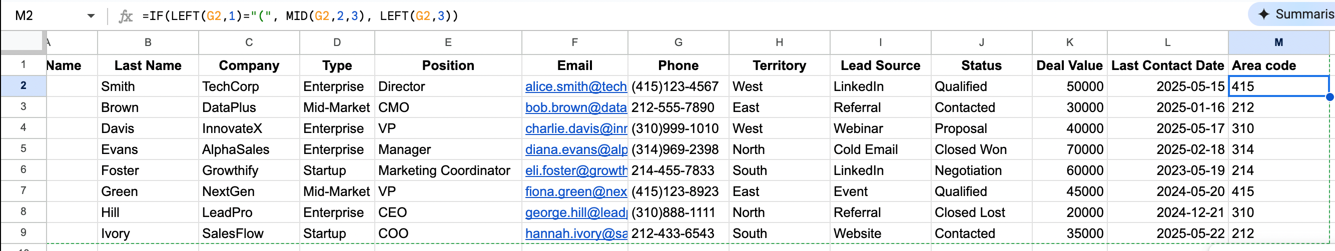
Sales example: Extract area codes from phone numbers for territory mapping:
=IF(LEFT(G2,1)="(", MID(G2,2,3), LEFT(G2,3))Extracts the area code whether the format is (123)456-7890 or 123-456-7890
Additional uses:
- Parse names from inconsistent formats
- Extract company identifiers from product codes
- Standardize address components
- Split domain names from email addresses
LEN: Verify the completeness of your prospect records
LEN helps you check text length, which is useful for verifying that data meets minimum requirements or identifying fields that need enrichment.
LEN syntax:
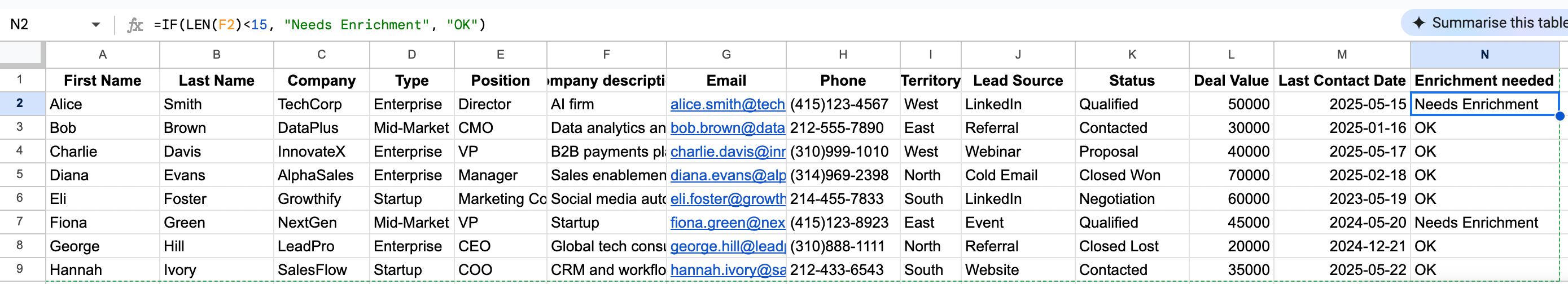
=LEN(text)Sales example: Flag incomplete contact records that need enrichment:
=IF(LEN(F2)<15, "Needs Enrichment", "OK")Marks records where the data in column D (e.g., company description) is too short
Additional uses:
- Verify phone numbers have the correct length
- Check that addresses meet minimum completeness
- Identify overly brief notes that need expansion
- Flag prospect records needing enrichment
MAX & MIN: Identify your best opportunities and biggest challenges
These functions find the maximum value and minimum value in a range, perfect for identifying outliers and setting benchmarks.
MAX & MIN syntax:
- =MAX(number1, [number2], …) – Returns the highest value
- =MIN(number1, [number2], …) – Returns the smallest value
=MAX(E2:E100)Returns the highest value from column E (deal values)
Additional uses:
- Find your longest sales cycle to identify process issues
- Identify your shortest time-to-close for best practice analysis
- Set benchmarks for performance tracking
- Highlight extreme values for special attention or analysis
- Use ABS to compare absolute value of gains/losses between periods
NETWORKDAYS: Calculate realistic sales cycle timeframes
NETWORKDAYS calculates working days between dates, giving you more accurate sales cycle projections by excluding weekends.
NETWORKDAYS syntax:
=NETWORKDAYS(start_date, end_date, [holidays])Sales example: Calculate actual working days in your sales cycle:
=NETWORKDAYS(C2, D2)Calculates working days between opportunity creation (C2) and the close date (D2)
Additional uses:
- Project realistic closing timeframes
- Set more accurate follow-up schedules
- Calculate average working days to close by deal type
- Measure response time in working days rather than calendar days
PIVOT TABLES: Analyze your sales performance from multiple Angles
While not a formula, pivot tables are essential for data analysis and sales analytics.
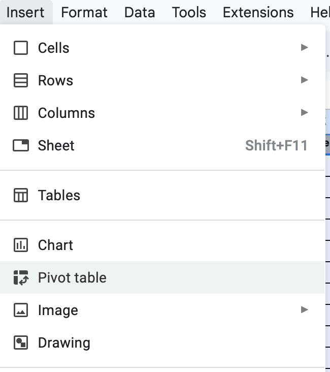
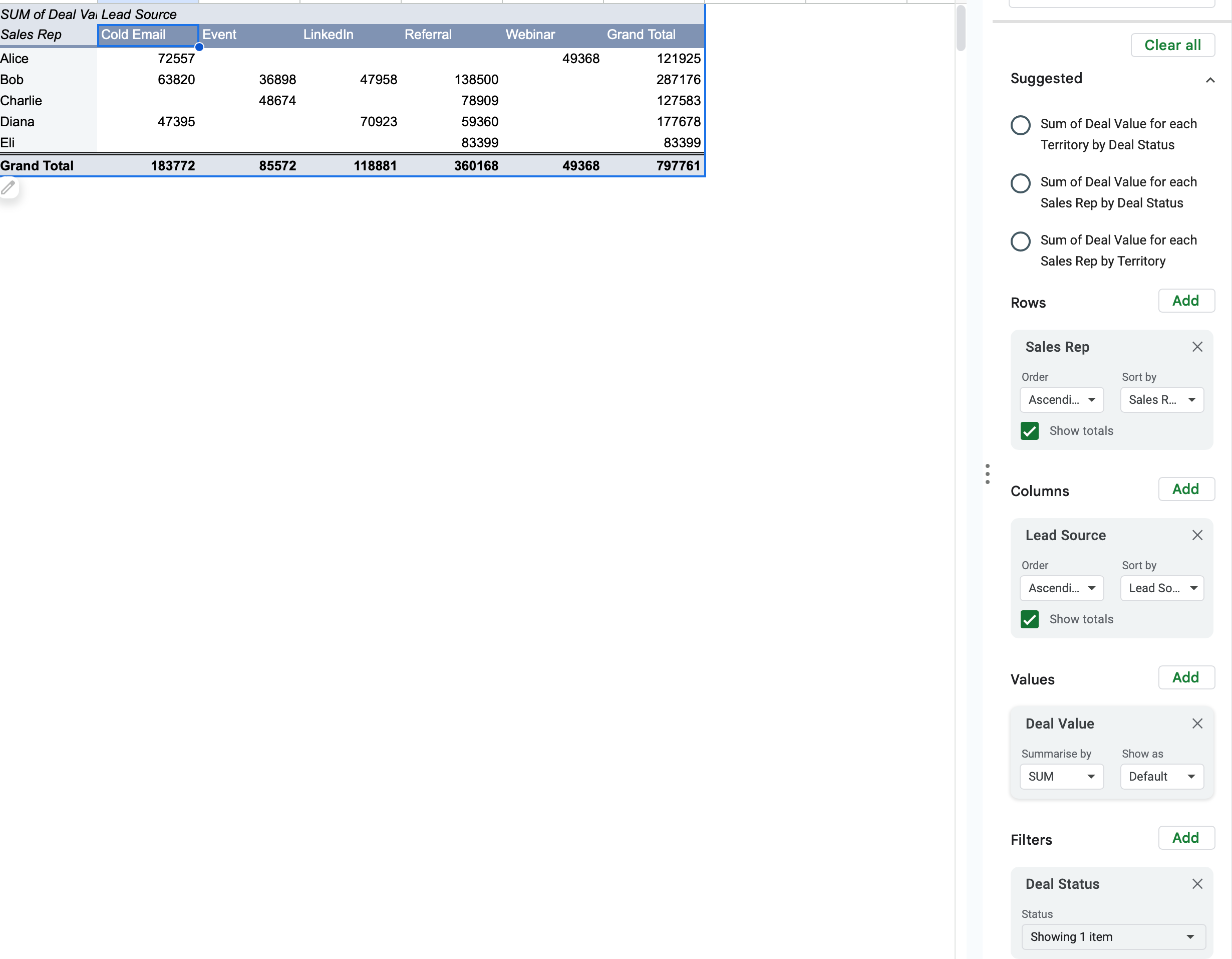
Sales example: Analyze closing rates by lead source and sales rep:
- Create a pivot table from your data by selecting your data, clicking on “Insert.” and then will choose “Pivot table.”
- Add “Sales Rep” to Rows
- Add “Lead Source” to Columns
- Add “Deal Status” to Filters and filter for “Closed Won”
- Add “Deal Value” to Values
Additional uses:
- Identify performance patterns across multiple dimensions
- Visualize territory performance by product and industry
- Analyze seasonal trends in sales metrics
- Compare team performance across different criteria
QUERY: Create custom sales reports with multiple conditions
QUERY lets you use SQL-like commands to manipulate data, perfect for creating flexible reports from complex sales data.
QUERY syntax:
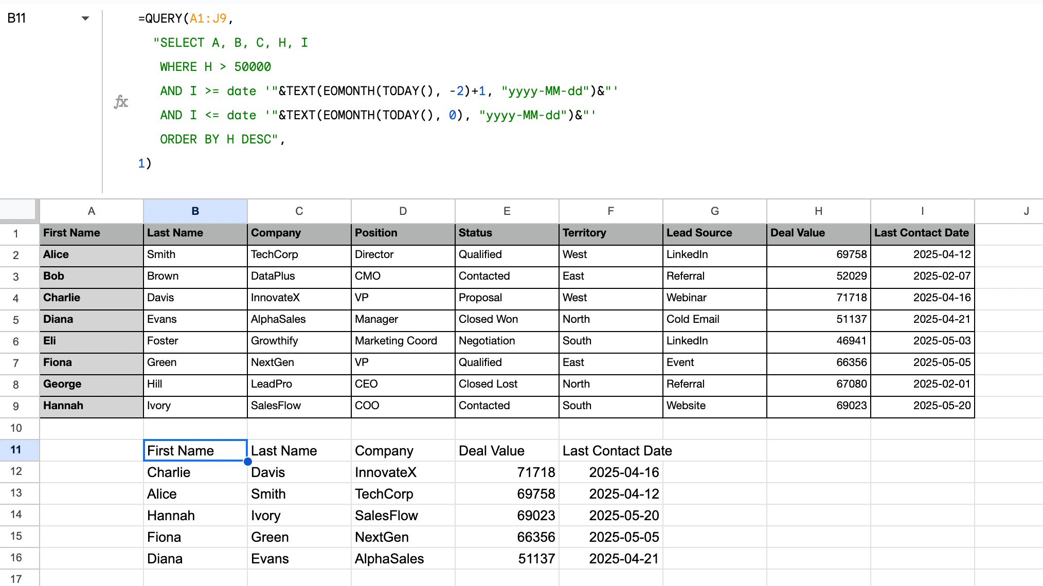
=QUERY(data, query, [headers])Sales example: Create a report of high-value opportunities closing this quarter:
=QUERY(A1:J9,
"SELECT A, B, C, H, I
 WHERE H > 50000
   AND I >= date '"&TEXT(EOMONTH(TODAY(), -2)+1, "yyyy-MM-dd")&"'
   AND I <= date '"&TEXT(EOMONTH(TODAY(), 0), "yyyy-MM-dd")&"'
 ORDER BY H DESC",
1)
Returns first name, last name, company, deal value, and last contact date for all opportunities with a deal value over $50k, closing within the current quarter.
Additional uses:
- Build flexible dashboards that respond to changing criteria
- Create automated weekly reports for management review
- Generate territory-specific analyses on demand
- Perform complex filtering operations based on multiple criteria
REGEXMATCH: Categorize prospects using pattern recognition
REGEXMATCH function uses regular expressions to identify patterns in text, perfect for advanced categorization and data cleaning.
REGEXMATCH syntax:
=REGEXMATCH(text, regular_expression)Sales example: Categorize prospects based on email domain patterns:
=IF(REGEXMATCH(E2, ".(edu|gov)$"), "Public Sector", IF(REGEXMATCH(E2, ".co.uk$"), "UK", "Commercial"))Categorizes email addresses ending in .edu or .gov as “Public Sector”, .co.uk as “UK”, and everything else as “Commercial”
Additional uses:
- Clean and standardize company names
- Identify industry segments based on terminology in descriptions
- Categorize job titles into management levels
- Flag specific keywords in prospect communication
SORT: Prioritize your prospects and opportunities automatically
SORT arranges data based on one or more columns, helping you create prioritized lists for outreach and follow-up.
SORT syntax:
=SORT(range, sort_column, is_ascending, [sort_column2, is_ascending2, ...])Sales example: Create a prioritized call list based on deal value and recency:
=SORT(A2:E50, 5, FALSE, 4, TRUE)Sorts data by column E (value) in descending order, then by column D (last contact) in ascending order
Additional uses:
- Organize prospects by engagement score
- Prioritize daily outreach activities
- Rank opportunities by close probability
- Create call lists based on multiple priority factors
SPARKLINE: Visualize deal progress and trends directly in your spreadsheet
SPARKLINE creates mini-charts inside cells, allowing you to see trends alongside your data without creating separate charts.
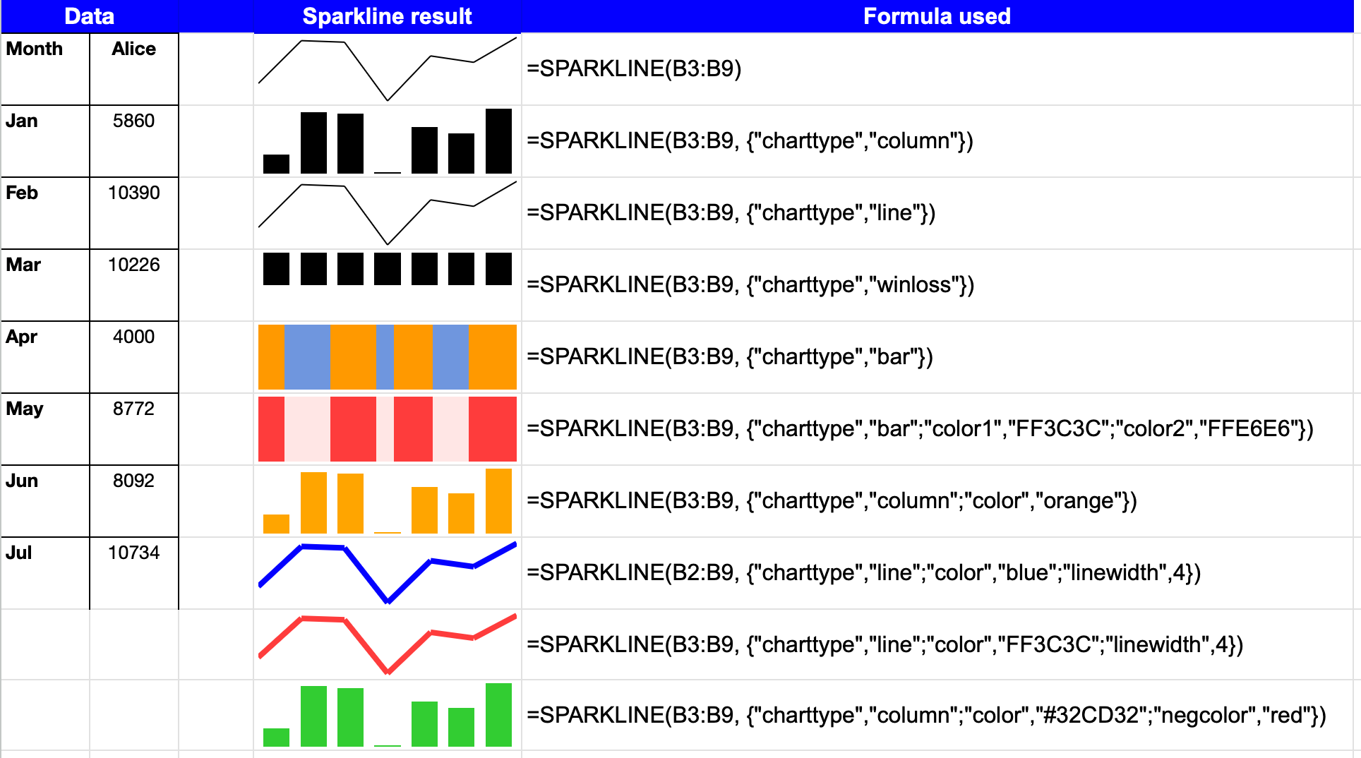
SPARKLINE syntax:
=SPARKLINE(data, [options])Sales example: Show monthly progress toward sales targets:
=SPARKLINE(B2:M2, {"charttype","bar")Creates a bar chart showing monthly sales.
Additional uses:
- Create mini trend visualizations of deal progress
- Show velocity metrics in-line with prospect data
- Visualize week-over-week activity metrics
- Display historical win rates alongside current opportunities
SUBSTITUTE: Clean and standardize imported contact data
SUBSTITUTE replaces specific text within strings (text data), perfect for cleaning and standardizing inconsistent data formats.
SUBSTITUTE syntax:
=SUBSTITUTE(text, old_text, new_text, [instance_num])Sales example: Standardize phone number formats:
=SUBSTITUTE(SUBSTITUTE(SUBSTITUTE(A2, "(", ""), ")", ""), "-", "")Removes parentheses and dashes from phone numbers to create a standardized format.
Additional uses:
- Clean formatting issues in imported prospect data
- Standardize inconsistent entry formats
- Normalize company name variations
- Replace abbreviations with full terms for consistency
SUM, SUMIF & SUMIFS: Calculate pipeline values and performance totals
These functions add up values based on various criteria, making them ideal for pipeline analysis and performance tracking.
SUM, SUMIF & SUMIFS syntax:
- =SUM(number1, [number2], …) – Adds all values
- =SUMIF(range, criteria, [sum_range]) – Adds values based on a condition
- =SUMIFS(sum_range, criteria_range1, criteria1, [criteria_range2, criteria2]…) – Adds values based on multiple conditions
Sales example: Calculate pipeline value by closing month:
=SUMIFS(F2:F100, E2:E100, "Qualified", D2:D100, ">="&DATE(YEAR(TODAY()),MONTH(TODAY()),1), D2:D100, "<"&EOMONTH(TODAY(),0)+1)Sums values from column F where status is “Qualified” (column E) and close date (column D) is in the current month.
Additional uses:
- Track activity metrics by sales rep
- Measure campaign performance by lead source
- Calculate pipeline value by stage and territory
- Analyze conversion values across different segments
TRIM: Prepare contact data for matching and analysis
TRIM removes extra spaces from text, fixing common issues with imported or manually entered data.
TRIM syntax:
=TRIM(text)Sales example: Clean up company names for consistent matching:
=TRIM(C2)Removes any leading, trailing, or extra spaces in the company name.
Additional uses:
- Clean up imported contact data with extra spaces
- Prepare data for matching operations
- Fix common formatting issues from copy-paste operations
- Standardize text entries for consistent analysis
UNIQUE: Remove Duplicate Contacts and Companies From Your Database
UNIQUE extracts distinct values from a range, helping you identify unique entries and remove duplicates.
UNIQUE syntax:
=UNIQUE(range)Sales example: Create a list of unique companies from your contact database:
=UNIQUE(C2:C200)Returns only unique company names from column C
Additional uses:
- Remove duplicate contacts from prospecting lists
- Create distinct company lists from contact databases
- Identify unique lead sources for analysis
- Extract unique values for dropdown lists in data validation
VLOOKUP, HLOOKUP & XLOOKUP: Match and Enrich Your Prospect Information
These lookup functions help you find and retrieve related information across different datasets, making them ideal for data enrichment.
VLOOKUP, HLOOKUP & XLOOKUP syntax:
- =VLOOKUP(lookup_value, table_array, col_index_num, [range_lookup]) – Vertical lookup
- =HLOOKUP(lookup_value, table_array, row_index_num, [range_lookup]) – Horizontal lookup
- =XLOOKUP(lookup_value, lookup_array, return_array, [if_not_found], [match_mode], [search_mode]) – Most flexible lookup
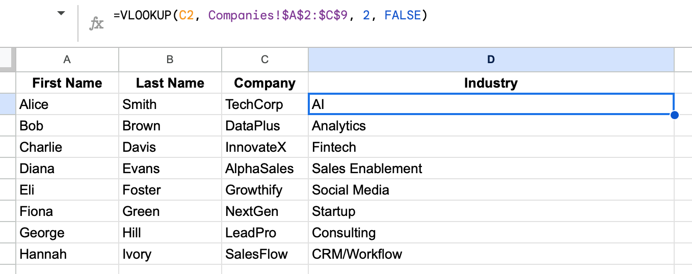
Sales example: Enrich contact records with company information:
=VLOOKUP(C2, Companies!$A$2:$C$9, 2, FALSELooks up the company name in C2 by matching it against the first column of the range Companies!$A$2:$C$9 in the Companies tab, and returns the corresponding industry from column 2.
Note: VLOOKUP always searches the first column of the range for a match—so in this case, the company names must be listed in column A of the Companies sheet.
Additional uses:
- Match inbound leads to existing accounts
- Pull in additional contact details from a master database
- Connect CRM IDs with internal tracking systems
- Link product details to opportunity records
Conditional formatting: Visualize your sales data for quick Insights
Conditional formatting transforms your sales data into a visual dashboard without creating separate charts. This powerful feature helps you identify patterns, spot warm leads, and flag items requiring attention.
Highlight deals that haven’t moved in 30+ days
How to set it up:
- Select your opportunity data range
- Go to Format > Conditional formatting
- Choose “Custom formula is” from the dropdown
- Enter: =TODAY()-$E2>30 (assuming E2 contains the “Last Updated” date)
- Set the formatting style (red background with white text works well)
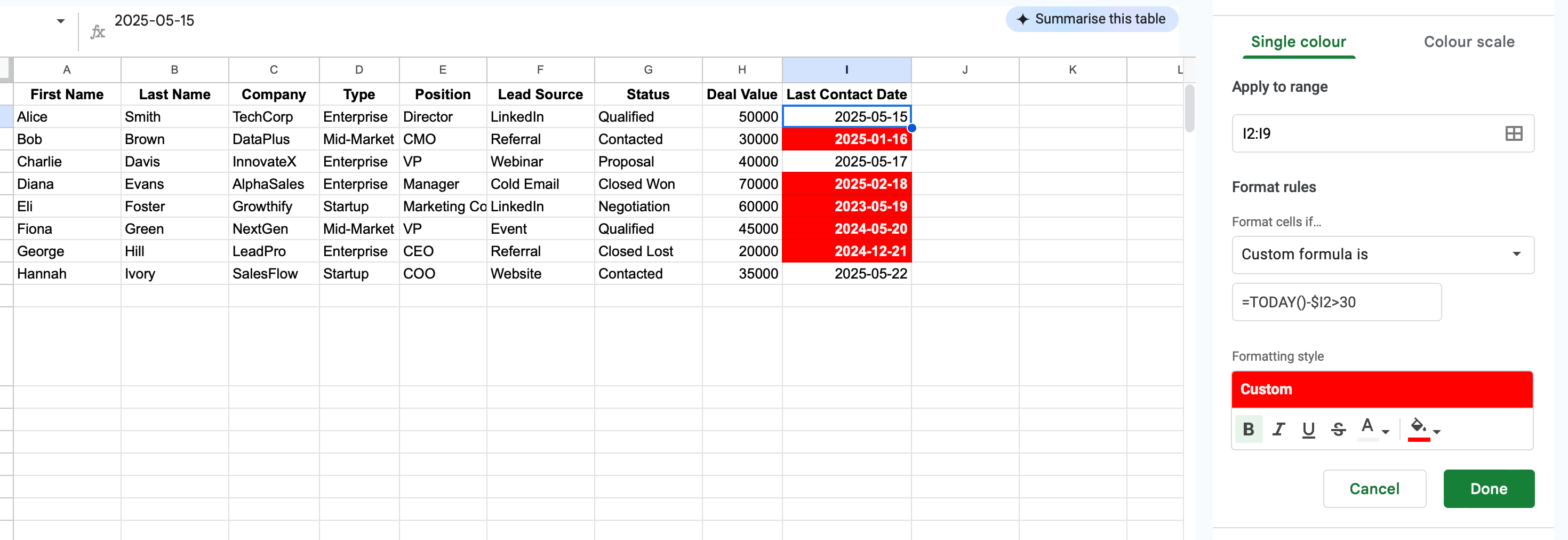
This visually flags any deals that haven’t seen activity in over a month, preventing opportunities from falling through the cracks.
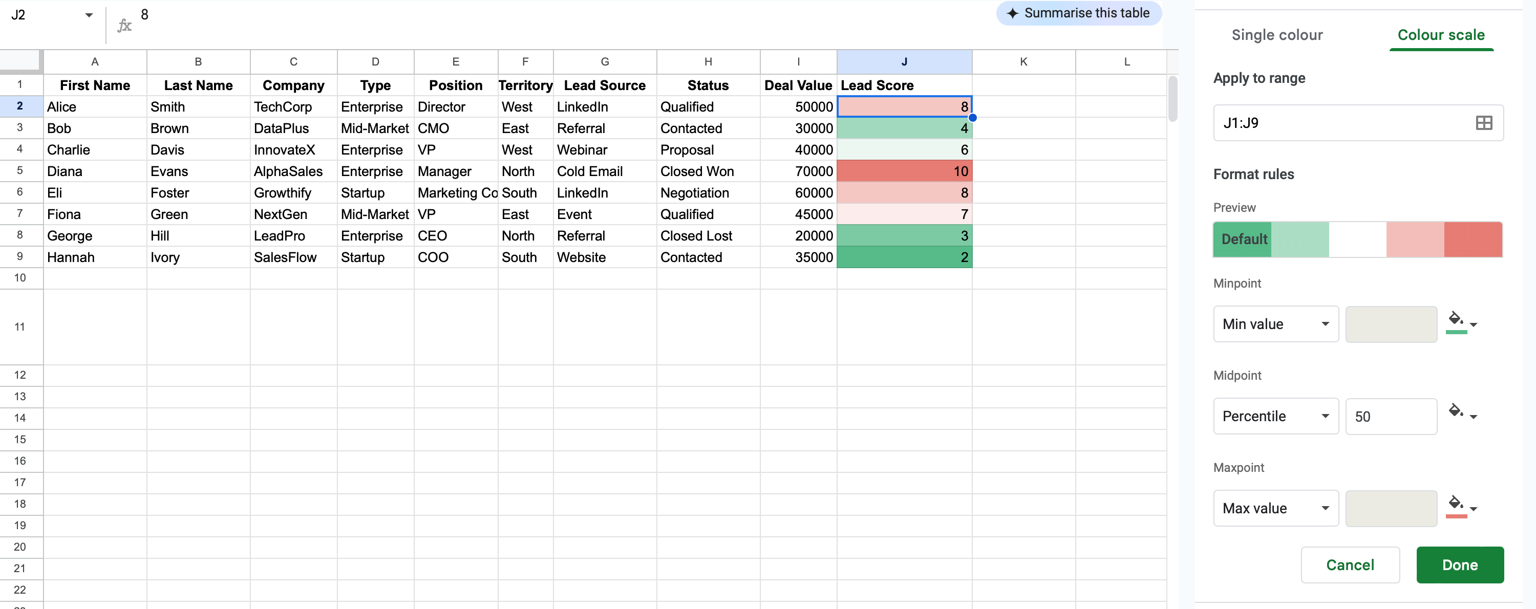
Color-code prospects based on lead score or engagement level
How to set it up:
- Select your lead score column
- Go to Format > Conditional formatting
- Choose “Color scale”
- Select a green-to-red scale (high scores green, low scores red)
Alternatively, create custom rules for score ranges:
- Choose “Custom formula is”
- For A-leads: =$F2>=80 with green background
- For B-leads: =AND($F2>=50,$F2<80) with yellow background
- For C-leads: =$F2<50 with red background
This creates an instant visual prioritization system for your prospect list.
Create heat maps of sales performance by rep or territory
How to set it up:
- Select your data range (reps in rows, months in columns, values in cells)
- Go to Format > Conditional formatting
- Choose “Color scale”
- Select a white-to-blue scale for a professional look
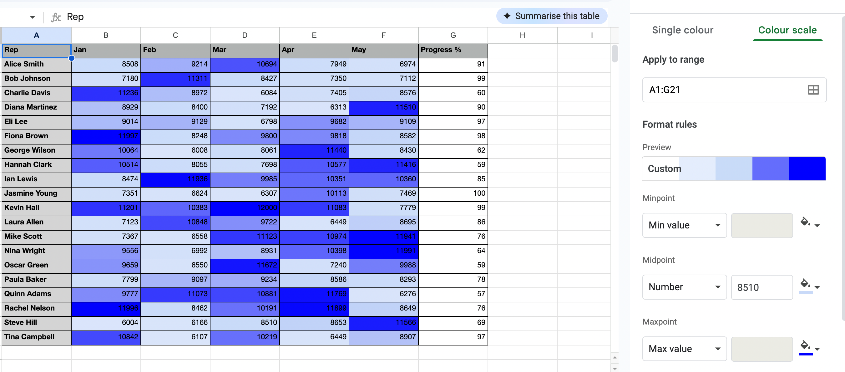
This instantly shows which reps are performing well (darker cells) and who might need coaching (lighter cells).
Google Sheets basics every sales rep should know
Best practices for organizing sales tracking spreadsheets
To manage your sales data efficiently, follow these core tips:
- Use separate sheets to organize and store data for prospects, pipeline, closed deals, and dashboards.
- Keep column names consistent across tabs (name, company, status, etc.).
- Freeze headers and key columns to keep key information visible while scrolling.
- Create reusable templates and duplicate them for each new month or quarter.
Formatting cells for better sales data visualization
| Formatting aspect | Best practices |
|---|---|
| Number Formats | Currency for deal values: Format > Number > Currency |
| Percentages for probabilities: Format > Number > Percent | |
| Custom number format for phone numbers: Format > Number > More Formats > Custom number format: (###) ###-#### | |
| Text Alignment | Left-align text and headers |
| Right-align number values | |
| Center status indicators | |
| Font Choices | 11pt for most data |
| 12pt bold for headers | |
| Use color sparingly (for status or highlighting only) | |
| Column Width Optimization | Double-click between column headers to auto-resize |
| Preset widths for standard columns (names, companies, etc.) |
How to use data validation for consistent lead entry and categorization
Data validation ensures your team enters standardized information, making analysis easier and more accurate.
To implement data validation, select your column, go to Data > Data validation, then choose either:
- Dropdown (from a range) to reference a column elsewhere (e.g., a list of deal stages)
- or Dropdown to manually enter predefined values (like “Qualified”, “Contacted”, etc.)
You can also enable the dropdown arrow and optional help text.
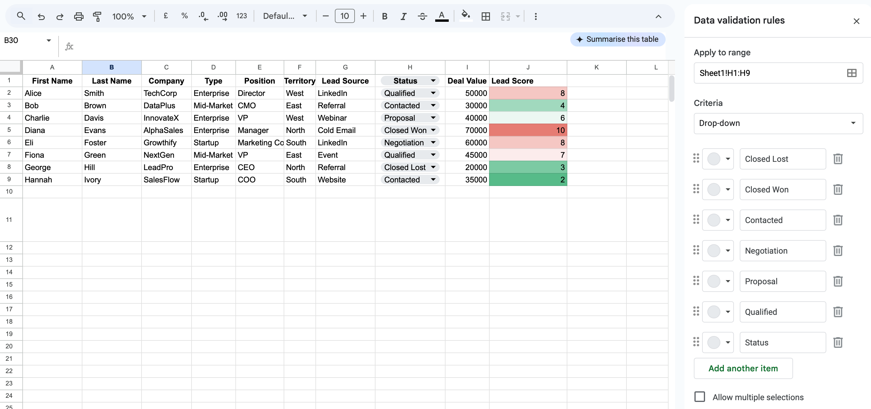
Sales-specific validation examples
- Lead status: Prospect, Qualified, Proposal, Negotiation, Closed Won, Closed Lost
- Lead source: Referral, LinkedIn, Website, Event, Cold Call, Partner
- Priority: A, B, C
- Industry: Technology, Healthcare, Finance, Manufacturing, Retail, etc.
This ensures data consistency, prevents typos, and makes filtering much more reliable.
How to set up protected ranges for sensitive sales information
How to protect sensitive data in Google Sheets: Select the cells you want to protect, right-click and choose “View more cell actions” > “Protect range.” Then adjust editing permissions to restrict access.
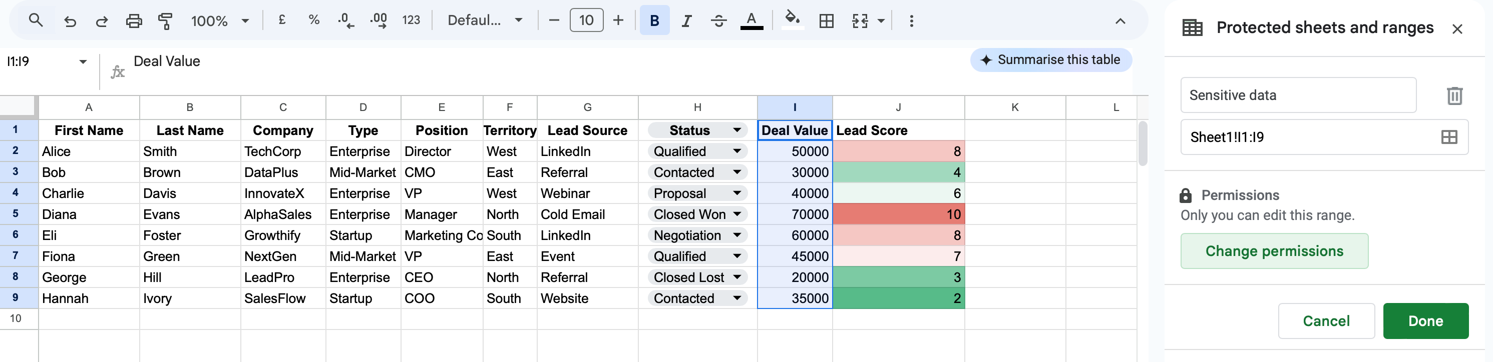
Sales information worth protecting
- Formulas calculating commissions
- Target and quota information
- Customer discount rates
- Data validation ranges
- Key dashboard calculations
This maintains formula integrity and prevents accidental edits to important fields.
Other useful Google Sheets functions & tips for sales teams
Whether you’re new to Google Sheets or looking to push its advanced features, there are plenty of lesser-known formulas and options that can enhance your data set and streamline daily operations.
Use these to improve your workflow:
- Use COLUMN() to return the column letter, or ROW() for the row number.
- CELL() returns the starting cell reference or cell range properties.
- Apply ROUND() or format options to control decimal value, decimal places, or simplify to the nearest integer of a specified number of digits.
- ISBLANK() flags empty cells while COUNTA() detects non-empty cells.
- Conditional formulas like IFS() or SWITCH() help when logic evaluates multiple conditions or filters by a specified range.
- Apply finance formulas like PMT() or IPMT() to calculate interest payment, periodic payment, periodic interest, and payment periods.
- Use GOOGLEFINANCE() to export historical securities information from Google Finance or create lightweight financial reports.
- Use RAND() or RANDBETWEEN() to generate a random number for simulations or testing.
- Use BASE(number, base) to convert numbers into a specified base, such as binary or hexadecimal.
- Use math functions like ABS(), SQRT() (for square root), or POWER() to perform quick calculations.
- Access the menu bar to create drop-downs, format cells, or automate with Google Workspace add-ons.
These tips bridge the gap between Excel basics and more powerful setups, even if you’re used to Microsoft Excel.
Google Sheets keyboard shortcuts for sales productivity
Speed up your daily sales data work with these time-saving shortcuts. Mastering these can significantly boost sales productivity and improve overall sales efficiency by saving hours of administrative time each week.
Navigation shortcuts to move efficiently through prospect lists
| Shortcut | Action | Sales use case |
|---|---|---|
| Ctrl + Home | Jump to the beginning of the sheet | Return to top of prospect list |
| Ctrl + End | Jump to the last cell with content | Skip to the end of your data |
| Ctrl + Arrow Key | Jump to the edge of a data region | Move between sections quickly |
| Alt + Down | Open the dropdown menu | Access lead status options |
| Ctrl + Page Down/Up | Switch between sheets | Move between pipeline stages |
| Ctrl + G | Go to a specific cell | Jump to specific prospect record |
| Ctrl + Shift + Arrow | Select the edge of the data | Select an entire prospect record |
Editing shortcuts for quick data updates
| Shortcut | Action | Sales use case |
|---|---|---|
| Ctrl + ; | Insert current date | Log contact dates instantly |
| F2 | Edit cell | Quick update to notes or status |
| Ctrl + Enter | Stay in the current cell after entry | Update multiple fields without clicking |
| Shift + Enter | Complete the entry and move up | Work backwards through a list |
| Ctrl + K | Insert hyperlink | Add links to LinkedIn profiles or proposals |
| Ctrl + Alt + V | Paste special | Paste only values from CRM without formatting |
| Alt + Enter | Add a line break within a cell | Format detailed notes cleanly |
Formatting shortcuts for consistent sales reporting
| Shortcut | Action | Sales use case |
|---|---|---|
| Ctrl + B | Bold | Highlight key prospects |
| Ctrl + Shift + 1 | Number format | Standardize number display |
| Ctrl + Shift + 4 | Currency format | Quick format deal values |
| Ctrl + Shift + 5 | Percentage format | Format conversion rates |
| Alt + H + H | Fill color | Status highlighting |
| Ctrl + Shift + F | Open format cells dialog | Advanced formatting options |
| Ctrl + Space | Select entire column | Format all status indicators at once |
Formula shortcuts to speed up analysis
| Shortcut | Action | Sales Use Case |
|---|---|---|
| = | Start formula | Begin any calculation |
| F4 | Toggle absolute/relative references | Lock territory or period references |
| Ctrl + Shift + Enter | Enter array formula | Apply lead scoring to multiple prospects |
| Alt + = | AutoSum | Quickly total your pipeline |
| Ctrl + ~ | Show formulas | Debug your sales calculations |
| Ctrl + Shift + U | Expand formula bar | Write complex prospect analysis formulas |
| Shift + F3 | Open function wizard | Get help with unfamiliar functions |
Importing and enriching sales data inside Google Sheets
Transform basic contact lists into rich prospect databases and keep your pipeline data fresh with streamlined enrichment techniques.
Bringing LinkedIn search results into your prospect sheets
You don’t need to manually copy results from LinkedIn into your spreadsheet. With PhantomBuster, you can pull them in automatically. Just run a LinkedIn search using the filters you already use — job title, location, industry — and the LinkedIn Search Export automation grabs the matching profiles for you.
The data goes straight into Google Sheets, clean and ready to use. You can even set it to update on a schedule, so your prospect list stays fresh without you having to think about it.
If you want to go further, you can enrich each profile with job details, emails or company info using the LinkedIn Profile Scraper. It’s a simple way to take what LinkedIn gives you and turn it into something actually usable.
Phantombuster provides powerful prospecting automation tools to extract and import LinkedIn search results directly into Google Sheets, creating fresh prospect lists with minimal manual effort.
Enriching basic contact lists with detailed professional information
Once your LinkedIn search results are in Google Sheets, you can enrich them with professional context to build a truly usable prospect list. Instead of working with just names and companies, you’ll get key insights like job titles, work experience, skills, and company details, all pulled automatically.
To do that, connect your sheet to the LinkedIn Profile Scraper automation. It pulls detailed information for each contact in bulk, so you can qualify leads, segment faster, and prep outreach without manual research. This step turns your list into a proper lead database, ready for scoring, routing, or messaging.
If you’re starting with an existing CRM or event list instead of a LinkedIn export, no problem. Use the LinkedIn Profile URL Finder to match those contacts to their LinkedIn profiles before enriching. That way, any list becomes a launchpad.
FAQ: Google Sheets for sales teams
How to share prospect sheets securely
Steps: Click the Share button at the top-right of your Google Sheet. Add your teammates’ email addresses to invite them. Set their permissions according to the level of access you want to grant: Editor can make changes, Commenter can leave feedback, and Viewer can only view the file.
Security tips: To keep your data safe, use “Restricted” access rather than allowing “Anyone with the link” to access the sheet. Consider adding expiration dates for temporary access to limit how long someone can view or edit the document. Use protected ranges to safeguard sensitive fields from accidental changes. Finally, regularly review and update access permissions to maintain control over who can view or edit your data.
How to use ChatGPT inside Google Sheets
What to do:
- Install a ChatGPT Sheets Add-on
- Go to Extensions > [Add-on Name]
- Use prompts like:
- =GPT(“Write a cold email for ” & A2)
- =GPT(“Analyze objection: ” & D2)
- =GPT(“Give 3 pain points for a ” & C2 & ” in ” & D2)
Perfect for quick outreach, call recaps, or lead insights—without leaving Sheets.
How to track the version history of Google Sheets data
Steps: To track the version history of your Google Sheets data, go to File > Version History> See Version History. From there, you can view edits by user and date, and restore old versions as needed.
How to connect Google Sheets to your CRM
|
CRM Platform |
Steps to integrate with Google Sheets |
|
Salesforce |
|
|
HubSpot |
|
|
Other options |
|